Inspecting results

An analysis returns a result, and writes its maps and tables to the output directory. This tutorial reads one result from end to end: the left hemisphere of the quick start, thickness against age and sex in 99 people. All the output below is what that run printed.

Printing a result

Printing a result lists the settings it ran with, the sample, and a summary of the data. QDECR prints the same list at the end of every run:

out
#> [call ] qdecr_fastlm call:                   [qdecr_fastlm(formula = qdecr_thickness ~ age + sex, data = pheno,id = "id", hemi = hemi, dir_out = results, project = "age_sex",n_cores = 4, dir_tmp = "/dev/shm", clobber = TRUE)]
#> [input] Hemisphere:                          [lh]
#> [input] Project name:                        [age_sex]
#> [input] Project final name:                  [lh.age_sex.thickness]
#> [input] Number of cores:                     [4]
#> [input] Target:                              [fsaverage]
#> [input] dir_out_tree:                        [TRUE]
#> [input] clobber:                             [TRUE]
#> [input] fwhm:                                [10]
#> [paths] Subjects dir:                        [/home/slamballais/qdecr-example/subjects]
#> [paths] Freesurfer home dir:                 [/home/slamballais/qdecr-example/freesurfer]
#> [paths] Temp dir:                            [/dev/shm]
#> [paths] Output dir:                          [/home/slamballais/qdecr-example/results/lh.age_sex.thickness]
#> [paths] Path to default mask:                [/home/slamballais/R/x86_64-pc-linux-gnu-library/4.5/QDECR/extdata/lh.fsaverage.cortex.mask.mgh]
#> [data ] N subjects:                          [99]
#> [data ] N data points:                       [99]
#> [data ] N datasets:                          [1]
#> [data ] Vertices loaded:                     [163842]
#> [model] Model:                               [RcppEigen::fastLm]
#> [model] Vertex data:                         [thickness]
#> [model] Formula:                             [qdecr_thickness ~ age + sex]
#> [model] Weights used:                        [No]
#> [mask ] Mask origin:                         [/home/slamballais/R/x86_64-pc-linux-gnu-library/4.5/QDECR/extdata/lh.fsaverage.cortex.mask.mgh]
#> [mask ] Masked vertices:                     [149955]
#> [stack] Stack 1:                             [(Intercept)]
#> [stack] Stack 2:                             [age]
#> [stack] Stack 3:                             [sexmale]
#> [post ] Final mask path:                     [/home/slamballais/qdecr-example/results/lh.age_sex.thickness/finalMask.mgh]
#> [post ] Final N vertices:                    [149953]
#> [post ] Estimated fwhm:                      [15]
#> [post ] Mean thickness per vertex:           [2.80535647037718]
#> [post ] SD thickness per vertex:             [0.355120966400878]
#> [post ] Mean thickness per subject:          [2.80535647037718]
#> [post ] SD thickness per subject:            [0.532521460331536]

Each line is tagged with what it describes:

The [post ] lines need a word each:

• Final N vertices is the mask the correction used. While estimating the smoothness, mris_fwhm prunes the odd vertex from the mask it was given, two here.
• Estimated fwhm is the smoothness of the residuals, rounded to the whole millimetre that picks FreeSurfer’s simulations: 15 mm. qdecr_fwhm(out) returns it.
• Mean thickness per vertex and per subject are the same number, the mean over all subjects and vertices, reached in two orders.
• SD thickness per vertex is the standard deviation across subjects at each vertex, averaged over the vertices: how much people differ at the same place, 0.36 mm. SD thickness per subject is the standard deviation across the cortex within each subject, averaged over the subjects: how much thickness varies from place to place, 0.53 mm.

The result answers the usual questions of a model, too: nobs(out) gives the number of subjects, and formula(out) the formula.

Summaries of the clusters

summary() lists every significant cluster of every stack, one row each, and with annot = TRUE the regions each covers most:

summary(out, annot = TRUE)
#>     variable cluster n_vertices mean_thickness mean_coefficient     mean_se                     top_region1                      top_region2                      top_region3
#>  (Intercept)       1     149953       2.805844       3.21187175 0.100971133   superiorfrontal (8.12%, 100%)         precentral (7.16%, 100%)   superiorparietal (6.97%, 100%)
#>          age       1     113272       2.806824      -0.02876963 0.005052009 superiorfrontal (9.87%, 91.78%) superiorparietal (9.07%, 98.25%) inferiorparietal (6.92%, 99.63%)

So the cluster for age holds 113,272 of the 149,953 vertices, and on average thickness drops 0.029 mm a year across it. The largest part of it, 9.9%, lies in the superior frontal gyrus, and it covers 92% of that region. A stack with no significant cluster, like sexmale here, has no row. The intercept’s cluster always covers the whole cortex and means nothing: ignore it.

The regions come from the Desikan-Killiany atlas, aparc.annot in the target’s label directory. file picks another annotation there, and regions how many to list:

summary(out, annot = TRUE, file = "aparc.a2009s.annot", regions = 5)

summary() returns a data frame, so it can be filtered, sorted or saved like any other. QDECR already saves the one with annot = TRUE in the output directory, as the tab-separated significant_clusters.txt.

FreeSurfer’s cluster table

mri_surfcluster, which finds the clusters, writes a table of its own for each stack, with things summary() leaves out: the area, the peak, and the cluster-wise p-value. The result knows where each stack’s table is:

writeLines(readLines(out$stack$cluster.summary[[2]]))

It opens with some forty lines on how the clusters were found. The last few, for age:

#> # Overall max 27.1634 at vertex 31360
#> # Overall min 0 at vertex 8
#> # NClusters          1
#> # FixMNI = 0
#> #
#> # ClusterNo  Max   VtxMax   Size(mm^2)  MNIX   MNIY   MNIZ    CWP    CWPLow    CWPHi   NVtxs    WghtVtx   Annot
#>    1       27.1634   31360  59037.43    -32.0  -77.4   32.6  0.00010  0.00000  0.00020  113272   960487.38  inferiorparietal

The header above it records the settings: CSD thresh 3.000000 is the cluster-forming threshold as −log₁₀(p), p < 0.001, and CW PValue Threshold: 0.025 is cwp_thr. Understanding the statistics explains both.

Histograms

hist() draws the distribution of the measure, as a first check that the data look like thickness should. By default it takes the mean of each vertex across subjects:

hist(out)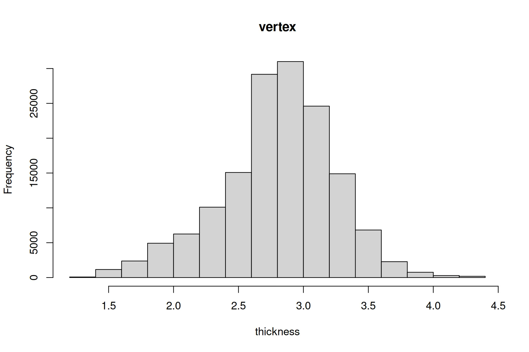

Thickness runs from about 1.5 to 4 mm across the cortex, which is right for adult and adolescent brains. Values near zero would mean vertices outside the cortex had crept into the mask; a second peak, a group of vertices unlike the rest.

With qtype = "subject" it takes the mean of each subject across the vertices instead:

hist(out, qtype = "subject")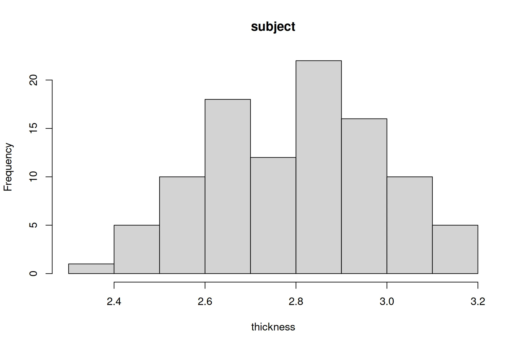

This is the one to look at for a subject whose processing went wrong: a failed surface, or a scan from someone else’s study, lands far from the rest. Here the subjects run from 2.3 to 3.2 mm, and none stands apart from the rest.

hist() passes anything else to R’s own hist(), so breaks, main and col work as usual.

Stacks

A stack is one coefficient of the model, with every map QDECR writes for it. stacks() lists them, in the order of the design matrix’s columns:

stacks(out)
#> [1] "(Intercept)" "age"         "sexmale"

The number is the stack’s place in that list, and it names the files in the output directory: stack 2 is age, so its t-statistic is stack2.t.mgh. Every function that takes a stack accepts the name or the number, so qdecr_snap(out, "age") and qdecr_snap(out, 2) draw the same map. Formulas and design explains how R names the columns, and Saving, loading and MGH files how to read a stack’s maps into R.