Plotting

QDECR draws its results with Freeview, FreeSurfer’s viewer, in two ways: qdecr_snap() has it take pictures of a map and returns them as one image, and freeview() opens the map in Freeview for you to explore. Both show a stack’s map on the inflated surface of the target, by default only inside its significant clusters. The figures here come from the left hemisphere of the quick start: thickness against age and sex in 99 people.

Snapshots with qdecr_snap

qdecr_snap() needs Freeview, a display for it to draw on, and the magick package to put the pictures together. Give it the result and a stack, by name or number:

img <- qdecr_snap(out, "age")
#> Opening Freeview on the command line. Pop-up incoming.
#> Call: freeview --surface /home/slamballais/qdecr-example/subjects/fsaverage/surf/lh.inflated:overlay=/dev/shm/lh.age_sex.thickness.stack2.temp_mgh.mgh:overlay_method=linearopaque:overlay_threshold=0.00810697115957737,0.0507556684315205 -cmd /dev/shm/tmp_snapshot_qdecr.txt
#> /dev/shm/tmp_snapshot_qdecr.txt contains: --viewport 3d --zoom 1 --ss /home/slamballais/qdecr-example/results/lh.age_sex.thickness.stack2.lateral.tiff --camera Azimuth 180 --ss /home/slamballais/qdecr-example/results/lh.age_sex.thickness.stack2.medial.tiff --camera Azimuth 180 --camera Elevation 90 --ss /home/slamballais/qdecr-example/results/lh.age_sex.thickness.stack2.superior.tiff --camera Elevation 180 --ss /home/slamballais/qdecr-example/results/lh.age_sex.thickness.stack2.inferior.tiff --quit
#> ERROR: label name '3rd-Ventricle' is duplicated!
#> ERROR: label name '3rd-Ventricle' is duplicated!
#> CTABfindDuplicateNames: 1 duplicate names found in:
#>   /tmp/FreeSurferColorLUT.txt
#> Executing commands from /dev/shm/tmp_snapshot_qdecr.txt

Freeview opens for a moment, takes a picture from each of four sides, and closes again; the lines after QDECR’s first three are Freeview’s own. The ERROR lines about 3rd-Ventricle are harmless: FreeSurfer 7.4.1’s Freeview complains about its own colour table on every start, and carries on. QDECR then crops the four pictures, puts them together and shows the result in R:

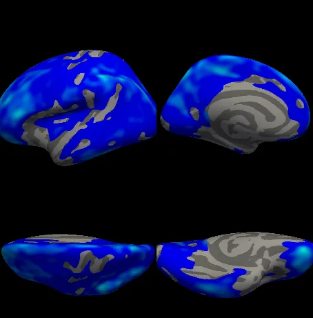
The pictures stay on disk, beside the output directory rather than in it: one per view and the composed one, named after the project and the stack’s number.

results/
├── lh.age_sex.thickness/
├── lh.age_sex.thickness.stack2.lateral.tiff
├── lh.age_sex.thickness.stack2.medial.tiff
├── lh.age_sex.thickness.stack2.superior.tiff
├── lh.age_sex.thickness.stack2.inferior.tiff
└── lh.age_sex.thickness.stack2.plot.tiff

qdecr_snap() also returns the composed image as a magick image, so it can be saved in another format or combined with others:

magick::image_write(img, "age.png", format = "png")

Which map

type picks the map: the coefficient ("coef", the default), its standard error ("se"), the t-statistic ("t") or the p-value as −log₁₀(p) ("p").

qdecr_snap(out, "age", type = "t")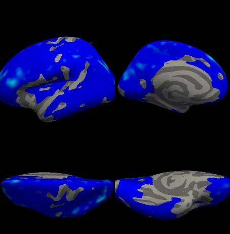

For age, the t-statistic looks much like the coefficient, because the effect is strong and the standard error about the same everywhere. Where they differ, the coefficient shows how large an effect is and the t-statistic how sure the model is of it.

The p-value map has no sign: a strong thinning and a strong thickening look the same. Take the direction from the coefficient or the t-statistic.

Colours

QDECR draws with Freeview’s heat scale: positive values in red to yellow, negative values in blue to cyan. The colours run from the smallest to the largest absolute value on show, so the palest blue marks the strongest thinning, and the scale differs from one picture to the next.

For pictures that compare, set the scale yourself, with Freeview’s own overlay_threshold: the value where colour starts, and the one where it saturates. Give overlay_method too, or QDECR replaces your threshold with its own:

qdecr_snap(out, "age", type = "p", overlay_method = "linearopaque", overlay_threshold = c(3, 10))

That draws −log₁₀(p) from 3, the cluster-forming threshold of p < 0.001, to 10, the scale of the picture on this site’s home page. Any other option of Freeview’s --surface flag works the same way, with its name as the argument: curvature_method, overlay_color and more; freeview --help lists them.

Other options

A stack without significant clusters has nothing to draw, and qdecr_snap() stops with “No information in the stack passed the threshold”: sexmale in this analysis, for one. Troubleshooting has more.

Without a screen

Freeview needs a display even to take pictures. On a server or a computing cluster, give it a virtual one with Xvfb, which is how the pictures on this site were made:

xvfb-run -a -s "-screen 0 1600x1200x24" Rscript snapshots.R

Freeview’s window sets the size of the pictures; under Xvfb here, the composed picture came out 454 pixels wide. On Windows 11, under WSL2, Freeview opens on the Windows desktop, and qdecr_snap() works as on Linux.

Opening Freeview

freeview() opens a stack’s map in Freeview, with the same choice of map and the same colours as qdecr_snap(), and leaves you in it:

freeview(out, "age")
freeview(out, "age", type = "t", sig = FALSE)

R waits until you close Freeview. In it you can turn and zoom the brain, click a vertex for its value, change the colour scale in the overlay’s settings, and switch to other surfaces. Freeview’s options pass through as they do for qdecr_snap().

Everything QDECR writes is a FreeSurfer file, so Freeview also opens the output directory without R. The p-value map masked to the significant clusters, and the clusters’ outlines as an annotation, on the inflated surface:

freeview -f "$SUBJECTS_DIR/fsaverage/surf/lh.inflated:overlay=results/lh.age_sex.thickness/stack2.cache.th30.abs.sig.masked.mgh:overlay_threshold=3,10:annot=results/lh.age_sex.thickness/stack2.cache.th30.abs.sig.ocn.annot:annot_outline=1"

Get started lists the files, and Saving, loading and MGH files how to read them into R for plots of your own.