Tutorial 1
Quick start
A complete analysis of cortical thickness against age and sex, from the data frame to the plot.
On this page
This tutorial runs one complete analysis of real data: cortical thickness against age and sex in 99 people aged 6 to 31. Every output on the page is what that run printed, and every figure is what it drew. The rest of the tutorials use the same analysis, so its results will look familiar there.
You need QDECR and FreeSurfer installed and working, as Get started describes. The run on this page used QDECR 0.9.0 with FreeSurfer 7.4.1 and R 4.5, in Ubuntu under WSL2. The scripts that reproduce it, from downloading the data to the figures, are in the repository.
The data
The scans come from ABIDE I, the Autism Brain Imaging Data Exchange, a public collection of MRI scans shared for research, as the Preprocessed Connectomes Project ran them through FreeSurfer, -qcache included. From its NYU site we took the typically developing participants, the ones without an autism diagnosis, less one whose scan failed the project’s quality check: 99 people aged 6.5 to 31.8, 26 of them female. The analysis leaves diagnosis out on purpose: the example shows what QDECR does, not a finding about autism.
Each participant has a directory in the subjects directory, named by their ID. QDECR reads a single file from it per hemisphere, the thickness map -qcache resampled to fsaverage and smoothed at 10 mm:
subjects/
├── fsaverage -> $FREESURFER_HOME/subjects/fsaverage
├── NYU_0051036/surf/lh.thickness.fwhm10.fsaverage.mgh
├── NYU_0051036/surf/rh.thickness.fwhm10.fsaverage.mgh
├── NYU_0051038/surf/...
└── ...
Those 198 files, 130 MB together, are all the imaging data the analysis needs. fsaverage, the target, is linked in from FreeSurfer, as Get started shows for subjects processed elsewhere.
The data frame has one row per participant. id holds the names of their directories, and sex becomes a factor with female first, so that the effect of sex is the difference of men from women:
library(QDECR)

pheno <- read.csv("phenotypes.csv")
pheno$sex <- factor(pheno$sex, levels = c("female", "male"))
head(pheno)
#>            id  age    sex site
#> 1 NYU_0051036 8.04 female  NYU
#> 2 NYU_0051038 8.26 female  NYU
#> 3 NYU_0051039 8.50 female  NYU
#> 4 NYU_0051040 8.52 female  NYU
#> 5 NYU_0051041 8.90 female  NYU
#> 6 NYU_0051042 8.91 female  NYU
QDECR finds the subjects through SUBJECTS_DIR, and so do the FreeSurfer tools it calls, so set it in the shell before R starts, as for FreeSurfer itself. The dir_subj argument points QDECR somewhere else, but not those tools: if you use it, keep the two the same.
Run the analysis
One call fits the model at every vertex of the left hemisphere and corrects for multiple testing:
out <- qdecr_fastlm(
  qdecr_thickness ~ age + sex,
  data = pheno,
  id = "id",
  hemi = "lh",
  project = "age_sex",
  dir_out = "results",
  dir_tmp = "/dev/shm",
  n_cores = 4
)
qdecr_thickness ~ age + sexis the model: thickness at each vertex, on age and sex. Theqdecr_prefix marks the vertex measure.projectnames the analysis. With the hemisphere and the measure it becomeslh.age_sex.thickness, the name of the output directory insideresults/.dir_tmp = "/dev/shm"keeps the large temporary files in memory, andn_cores = 4spreads the work over four processes. Performance and memory explains both.
QDECR reports each stage as it goes. It begins like this, the four starting worker lines being the processes n_cores asked for:
#> ------------------------------------------------------------
#> ----------------------- QDECR v0.9.0 -----------------------
#> ------------------------------------------------------------
#>
#> Welcome to QDECR (v0.9.0)
#> Authors: Sander Lamballais & Ryan Muetzel
#> Website: www.qdecr.com
#> Repository: www.github.com/slamballais/QDECR
#>
#> ------------------------------------------------------------
#> --------------------- Integrity checks ---------------------
#> ------------------------------------------------------------
#>
#> Checked all input arguments.
#>
#> ------------------------------------------------------------
#> ------------------- Loading vertex data --------------------
#> ------------------------------------------------------------
#>
#> starting worker pid=1236 on localhost:11324 at 10:43:57.267
#> starting worker pid=1237 on localhost:11324 at 10:43:57.281
#> starting worker pid=1238 on localhost:11324 at 10:43:57.294
#> starting worker pid=1239 on localhost:11324 at 10:43:57.307
#> loaded QDECR and set parent environment
#> loaded QDECR and set parent environment
#> loaded QDECR and set parent environment
#> loaded QDECR and set parent environment
#>   |==============================================================================================================================================================================================| 100%
After loading the vertex data it fits the model at the 149,955 vertices of the cortex, estimates how smooth the residuals are with FreeSurfer’s mris_fwhm, and hands each coefficient’s map to mri_surfcluster for the cluster-wise correction. Both FreeSurfer tools print a good deal on the way. On four cores the whole run took 61 seconds.
Look at the results
out is the result: the settings, the sample and a summary of the data, with the maps left on disk. Printing it gives the overview:
out
#> [call ] qdecr_fastlm call:                   [qdecr_fastlm(formula = qdecr_thickness ~ age + sex, data = pheno,id = "id", hemi = hemi, dir_out = results, project = "age_sex",n_cores = 4, dir_tmp = "/dev/shm", clobber = TRUE)]
#> [input] Hemisphere:                          [lh]
#> [input] Project name:                        [age_sex]
#> [input] Project final name:                  [lh.age_sex.thickness]
#> [input] Number of cores:                     [4]
#> [input] Target:                              [fsaverage]
#> [input] dir_out_tree:                        [TRUE]
#> [input] clobber:                             [TRUE]
#> [input] fwhm:                                [10]
#> [paths] Subjects dir:                        [/home/slamballais/qdecr-example/subjects]
#> [paths] Freesurfer home dir:                 [/home/slamballais/qdecr-example/freesurfer]
#> [paths] Temp dir:                            [/dev/shm]
#> [paths] Output dir:                          [/home/slamballais/qdecr-example/results/lh.age_sex.thickness]
#> [paths] Path to default mask:                [/home/slamballais/R/x86_64-pc-linux-gnu-library/4.5/QDECR/extdata/lh.fsaverage.cortex.mask.mgh]
#> [data ] N subjects:                          [99]
#> [data ] N data points:                       [99]
#> [data ] N datasets:                          [1]
#> [data ] Vertices loaded:                     [163842]
#> [model] Model:                               [RcppEigen::fastLm]
#> [model] Vertex data:                         [thickness]
#> [model] Formula:                             [qdecr_thickness ~ age + sex]
#> [model] Weights used:                        [No]
#> [mask ] Mask origin:                         [/home/slamballais/R/x86_64-pc-linux-gnu-library/4.5/QDECR/extdata/lh.fsaverage.cortex.mask.mgh]
#> [mask ] Masked vertices:                     [149955]
#> [stack] Stack 1:                             [(Intercept)]
#> [stack] Stack 2:                             [age]
#> [stack] Stack 3:                             [sexmale]
#> [post ] Final mask path:                     [/home/slamballais/qdecr-example/results/lh.age_sex.thickness/finalMask.mgh]
#> [post ] Final N vertices:                    [149953]
#> [post ] Estimated fwhm:                      [15]
#> [post ] Mean thickness per vertex:           [2.80535647037718]
#> [post ] SD thickness per vertex:             [0.355120966400878]
#> [post ] Mean thickness per subject:          [2.80535647037718]
#> [post ] SD thickness per subject:            [0.532521460331536]
The call reads hemi = hemi and dir_out = results because the run on this site looped over both hemispheres, with clobber = TRUE so it could be repeated over its own results. The smoothness of the residuals came out at 15 mm, higher than the 10 mm the data were smoothed with, which is usual for anatomical data. Inspecting results goes through the rest line by line.
The model has three coefficients, so the result has three stacks, each with its own maps and its own clusters:
stacks(out)
#> [1] "(Intercept)" "age"         "sexmale"
summary() lists the significant clusters, and with annot = TRUE the regions of the Desikan-Killiany atlas they cover most:
summary(out, annot = TRUE)
#>     variable cluster n_vertices mean_thickness mean_coefficient     mean_se                     top_region1                      top_region2                      top_region3
#>  (Intercept)       1     149953       2.805844       3.21187175 0.100971133   superiorfrontal (8.12%, 100%)         precentral (7.16%, 100%)   superiorparietal (6.97%, 100%)
#> age 1 113272 2.806824 -0.02876963 0.005052009 superiorfrontal (9.87%, 91.78%) superiorparietal (9.07%, 98.25%) inferiorparietal (6.92%, 99.63%)- Age has one significant cluster, 113,272 vertices and 59,037 mm², three quarters of the cortex. Its mean coefficient is −0.029: across the cluster, the cortex is 0.029 mm thinner for each year of age, about 0.7 mm between the youngest participant and the oldest, on a mean thickness of 2.8 mm. The cortex thins through childhood and adolescence, and on a sample this size the effect is hard to miss.
- Sex,
sexmale, has no row: no cluster of it survived the correction. - The intercept always covers the whole cortex, because it tests whether thickness is zero. It has no meaning here; ignore it.
In each region, the first percentage is how much of the cluster lies in that region, and the second how much of the region the cluster covers.
Plot the clusters
qdecr_snap() has Freeview draw a stack’s map on the inflated surface of fsaverage, only where the clusters are significant, from four sides, and puts the four views together. It needs Freeview and a display to draw on, and the magick package:
qdecr_snap(out, "age")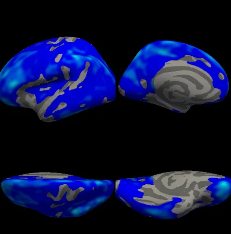
Blue marks a negative coefficient: thinner with age. The grey patches are the vertices outside the cluster, the medial wall among them, which has no cortex to measure. Plotting covers the other maps, the colours and Freeview itself.
Both hemispheres
One analysis covers one hemisphere, so a whole-brain study runs twice. The default cluster-wise threshold, cwp_thr = 0.025, is already 0.05 split over the two:
for (hemi in c("lh", "rh")) {
  out <- qdecr_fastlm(
    qdecr_thickness ~ age + sex,
    data = pheno, id = "id", hemi = hemi, project = "age_sex",
    dir_out = "results", dir_tmp = "/dev/shm", n_cores = 4
  )
  print(summary(out, annot = TRUE))
}
The right hemisphere tells the same story: one cluster for age, 117,846 vertices and 61,169 mm², with a mean coefficient of −0.029, and none for sex.
summary(out, annot = TRUE)
#>     variable cluster n_vertices mean_thickness mean_coefficient     mean_se                     top_region1                       top_region2                      top_region3
#>  (Intercept)       1     149926       2.814483       3.22835196 0.100551108   superiorfrontal (7.92%, 100%)          precentral (7.14%, 100%)   superiorparietal (6.82%, 100%)
#>          age       1     117846       2.814567      -0.02918288 0.005026116 superiorfrontal (9.63%, 95.59%) superiorparietal (8.67%, 100.00%) inferiorparietal (7.94%, 96.68%)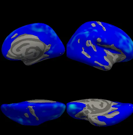
Where to go next
- Inspecting results: everything
print()andsummary()show, FreeSurfer’s own cluster table, and the histograms. - Plotting: the other maps, the colour scale, and Freeview.
- Formulas and design: what else the model can say.
- Understanding the statistics: what the correction does, and why the smoothness matters.